Tutorial 2: ATAC-RNA-Seq Mouse Brain RNA and ATAC Multi-Omics Data
We applied COSMOS to analyze a spatially resolved multi-omics dataset based on real-world experiments instead of simulated data. This experimental dataset contains P22 mouse brain coronal sections with a joint profiling of spatial chromatin accessibility (ATAC) and spatial transcriptome (RNA). The annotation was manually generated by aligning the sample with the P56 mouse brain coronal section from Allen Mouse Brain Atlas.
The raw data can be downloaded from: https://brain-spatial-omics.cells.ucsc.edu
The processed data is available at: https://zenodo.org/records/13932144
[1]:
import pandas as pd
import numpy as np
import scanpy as sc
import matplotlib
import matplotlib.pyplot as plt
from umap import UMAP
import sklearn
import seaborn as sns
from COSMOS import cosmos
from COSMOS.pyWNN import pyWNN
import h5py
import warnings
warnings.filterwarnings('ignore')
random_seed = 20
/Applications/anaconda3/envs/spaceflow_env/lib/python3.7/site-packages/tqdm/auto.py:21: TqdmWarning: IProgress not found. Please update jupyter and ipywidgets. See https://ipywidgets.readthedocs.io/en/stable/user_install.html
  from .autonotebook import tqdm as notebook_tqdm
Preparation of data
Importing the data
[2]:
data_mat = h5py.File('./ATAC_RNA_Seq_MouseBrain_RNA_ATAC.h5', 'r')
df_data_RNA = np.array(data_mat['X_RNA']).astype('float64')     # gene count matrix
df_data_ATAC= np.array(data_mat['X_ATAC']).astype('float64')  # protein count matrix
loc = np.array(data_mat['Pos']).astype('float64')
LayerName = list(data_mat['LayerName'])
LayerName = [item.decode("utf-8") for item in LayerName]

adata1 = sc.AnnData(df_data_RNA, dtype="float64")
adata1.obsm['spatial'] = np.array(loc)
adata1.obs['LayerName'] = LayerName
adata1.obs['x_pos'] = np.array(loc)[:,0]
adata1.obs['y_pos'] = np.array(loc)[:,1]

adata2 = sc.AnnData(df_data_ATAC, dtype="float64")
adata2.obsm['spatial'] = np.array(loc)
adata2.obs['LayerName'] = LayerName
adata2.obs['x_pos'] = np.array(loc)[:,0]
adata2.obs['y_pos'] = np.array(loc)[:,1]
Visualizing spatial positions with annotation
[3]:
adata_new = adata1.copy()
adata_new.obs["LayerName"]=adata_new.obs["LayerName"].astype('category')


matplotlib.rcParams['font.size'] = 12.0
fig, axes = plt.subplots(1, 1, figsize=(3.5,3))
sz = 20
plot_color=['#D1D1D1','#e6194b', '#3cb44b', '#ffe119', '#4363d8', '#f58231', '#911eb4', '#46f0f0', '#f032e6', \
            '#bcf60c', '#fabebe', '#008080', '#e6beff', '#9a6324', '#ffd8b1', '#800000', '#aaffc3', '#808000', '#000075', '#000000', '#808080', '#ffffff', '#fffac8']

domains="LayerName"
num_celltype=len(adata_new.obs[domains].unique())
adata_new.uns[domains+"_colors"]=list(plot_color[:num_celltype])
titles = 'Annotation '
ax=sc.pl.scatter(adata_new,alpha=1,x="x_pos",y="y_pos",color=domains,title=titles ,color_map=plot_color,show=False,size=sz,ax = axes)
ax.axis('off')
[3]:
(-4.95, 103.95, -2.8500000000000005, 103.85)

Applying COSMOS to integrate RNA and ATAC omics
[4]:
## COSMOS training
cosmos_comb = cosmos.Cosmos(adata1=adata1,adata2=adata2)
cosmos_comb.preprocessing_data(n_neighbors = 10)
cosmos_comb.train(spatial_regularization_strength=0.01, z_dim=50,
         lr=1e-3, wnn_epoch = 500, total_epoch=1000, max_patience_bef=10, max_patience_aft=30, min_stop=200,
         random_seed=random_seed, gpu=0, regularization_acceleration=True, edge_subset_sz=1000000)
weights = cosmos_comb.weights
df_embedding = pd.DataFrame(cosmos_comb.embedding)
Epoch 1/1000, Loss: 1.4096118211746216
Epoch 11/1000, Loss: 1.1203821897506714
Epoch 21/1000, Loss: 0.7638721466064453
Epoch 31/1000, Loss: 0.4149342179298401
Epoch 41/1000, Loss: 0.17488263547420502
Epoch 51/1000, Loss: 0.06789164245128632
Epoch 61/1000, Loss: 0.0332467220723629
Epoch 71/1000, Loss: 0.02090390771627426
Epoch 81/1000, Loss: 0.01618310436606407
Epoch 91/1000, Loss: 0.012922131456434727
Epoch 101/1000, Loss: 0.010959653183817863
Epoch 111/1000, Loss: 0.010975166223943233
Epoch 121/1000, Loss: 0.008905645459890366
Epoch 131/1000, Loss: 0.009921539574861526
Epoch 141/1000, Loss: 0.008092425763607025
Epoch 151/1000, Loss: 0.007676845416426659
Epoch 161/1000, Loss: 0.007937170565128326
Epoch 171/1000, Loss: 0.00713766273111105
Epoch 181/1000, Loss: 0.006691939663141966
Epoch 191/1000, Loss: 0.006564016919583082
Epoch 201/1000, Loss: 0.0060991630889475346
Epoch 211/1000, Loss: 0.005894108675420284
Epoch 221/1000, Loss: 0.005854759365320206
Epoch 231/1000, Loss: 0.00644934456795454
Computing KNN distance matrices using default Scanpy implementation
Computing modality weights
Computing weighted distances for union of 200 nearest neighbors between modalities
0 out of 9215 0.01 seconds elapsed
2000 out of 9215 14.91 seconds elapsed
4000 out of 9215 33.62 seconds elapsed
6000 out of 9215 50.52 seconds elapsed
8000 out of 9215 66.17 seconds elapsed
Selecting top K neighbors
Epoch 241/1000, Loss: 0.00976722501218319
Epoch 251/1000, Loss: 0.008706186898052692
Epoch 261/1000, Loss: 0.0083543062210083
Epoch 271/1000, Loss: 0.007722612004727125
Epoch 281/1000, Loss: 0.006718369200825691
Epoch 291/1000, Loss: 0.006474517751485109
Epoch 301/1000, Loss: 0.006135233677923679
Epoch 311/1000, Loss: 0.005993305705487728
Epoch 321/1000, Loss: 0.005595795810222626
Epoch 331/1000, Loss: 0.006280450150370598
Epoch 341/1000, Loss: 0.005268147215247154
Epoch 351/1000, Loss: 0.005161567125469446
Epoch 361/1000, Loss: 0.00490208063274622
Epoch 371/1000, Loss: 0.0049283732660114765
Epoch 381/1000, Loss: 0.005684142000973225
Epoch 391/1000, Loss: 0.004497723188251257
Epoch 401/1000, Loss: 0.004536759108304977
Epoch 411/1000, Loss: 0.004365301690995693
Epoch 421/1000, Loss: 0.004128994420170784
Epoch 431/1000, Loss: 0.0042103361338377
Epoch 441/1000, Loss: 0.004210502374917269
Epoch 451/1000, Loss: 0.003974263556301594
Epoch 461/1000, Loss: 0.003947787452489138
Epoch 471/1000, Loss: 0.0037678773514926434
Epoch 481/1000, Loss: 0.003693088423460722
Epoch 491/1000, Loss: 0.0037871231324970722
Epoch 501/1000, Loss: 0.0035643766168504953
Epoch 511/1000, Loss: 0.0034569408744573593
Epoch 521/1000, Loss: 0.003453570883721113
Epoch 531/1000, Loss: 0.0034160902723670006
Epoch 541/1000, Loss: 0.0036303717643022537
Epoch 551/1000, Loss: 0.0034599590580910444
Epoch 561/1000, Loss: 0.0034072331618517637
Epoch 571/1000, Loss: 0.0031724791042506695
Epoch 581/1000, Loss: 0.003167568240314722
Epoch 591/1000, Loss: 0.0031775173265486956
Epoch 601/1000, Loss: 0.003394388360902667
Epoch 611/1000, Loss: 0.003301542019471526
Epoch 621/1000, Loss: 0.003027899656444788
Epoch 631/1000, Loss: 0.0029416850302368402
Epoch 641/1000, Loss: 0.0030105530750006437
Epoch 651/1000, Loss: 0.0028281831182539463
Epoch 661/1000, Loss: 0.0029806550592184067
Epoch 671/1000, Loss: 0.0028709787875413895
Epoch 681/1000, Loss: 0.0028544238302856684
Epoch 691/1000, Loss: 0.004297688137739897
Epoch 701/1000, Loss: 0.0029091904871165752
Epoch 711/1000, Loss: 0.0027824100106954575
Epoch 721/1000, Loss: 0.002913344418630004
Epoch 731/1000, Loss: 0.0028275884687900543
Epoch 741/1000, Loss: 0.002887941198423505
Epoch 751/1000, Loss: 0.002716190880164504
Epoch 761/1000, Loss: 0.002677301410585642
Epoch 771/1000, Loss: 0.002753929700702429
Epoch 781/1000, Loss: 0.002718151779845357
Epoch 791/1000, Loss: 0.002680630888789892
Epoch 801/1000, Loss: 0.0026806769892573357
Epoch 811/1000, Loss: 0.0029179449193179607
Epoch 821/1000, Loss: 0.0025795595720410347
Epoch 831/1000, Loss: 0.002561993198469281
Epoch 841/1000, Loss: 0.0025949659757316113
Epoch 851/1000, Loss: 0.0025220406241714954
Epoch 861/1000, Loss: 0.002628563204780221
Epoch 871/1000, Loss: 0.002526515629142523
Epoch 881/1000, Loss: 0.002525521442294121
Epoch 891/1000, Loss: 0.0027280000504106283
Epoch 901/1000, Loss: 0.0025486331433057785
Epoch 911/1000, Loss: 0.0025585724506527185
Epoch 921/1000, Loss: 0.0025136114563792944
Epoch 931/1000, Loss: 0.0024391249753534794
Epoch 941/1000, Loss: 0.002414568094536662
Clustering of COSMOS integration
[5]:
adata_new = adata1.copy()
embedding_adata = sc.AnnData(df_embedding)
sc.pp.neighbors(embedding_adata, n_neighbors=50, use_rep='X')

# Manualy setting resolution for clustering
res = 1.0
sc.tl.louvain(embedding_adata, resolution=res)
adata_new.obs['Cluster_cosmos'] = list(embedding_adata.obs["louvain"].cat.codes)
adata_new.obs["Cluster_cosmos"]=adata_new.obs["Cluster_cosmos"].astype('category')

# Relabeling clusters with layer names
digit_labels = list(adata_new.obs['Cluster_cosmos'])
for i in range(len(digit_labels)):
    if digit_labels[i] not in [0,1,2,4,5,6,7,8,11]:
        digit_labels[i] = 100
adata_new.obs['Cluster_cosmos'] = digit_labels
adata_new.obs["Cluster_cosmos"]=adata_new.obs["Cluster_cosmos"].astype('category')
adata_new.obs['Cluster_cosmos'].cat.rename_categories({0: 'CP2',
                                                   1: 'L5',
                                                   2: 'CP1',
                                                   4: 'L4',
                                                   5: 'ccg/aco',
                                                   6: 'ACB',
                                                   7: 'L1-L3',
                                                    8: 'L6a/b',
                                                   11: 'VL',
                                                    100: '1_others'
                                                         }, inplace=True)

ordered_cluster = np.unique(list(adata_new.obs['Cluster_cosmos']))
adata_new.obs['Cluster_cosmos'] = adata_new.obs['Cluster_cosmos'].cat.reorder_categories(ordered_cluster, ordered=True)

# Calculating ARI
opt_cluster_cosmos = list(adata_new.obs['Cluster_cosmos'])
opt_ari_cosmos = sklearn.metrics.adjusted_rand_score(LayerName, opt_cluster_cosmos)
opt_ari_cosmos = round(opt_ari_cosmos, 2)

# Ploting figures
matplotlib.rcParams['font.size'] = 8.0
fig, axes = plt.subplots(1, 2, figsize=(6,2))
sz = 10
plot_color=['#D1D1D1','#e6194b', '#3cb44b', '#ffe119', '#4363d8', '#f58231', '#911eb4', '#46f0f0', '#f032e6', \
            '#bcf60c', '#fabebe', '#008080', '#e6beff', '#9a6324', '#ffd8b1', '#800000', '#aaffc3', '#808000', '#000075', '#000000', '#808080', '#ffffff', '#fffac8']
domains="LayerName"
num_celltype=len(adata_new.obs[domains].unique())
adata_new.uns[domains+"_colors"]=list(plot_color[:num_celltype])
titles = 'Annotation'
ax=sc.pl.scatter(adata_new,alpha=1,x="x_pos",y="y_pos",color=domains,title=titles ,color_map=plot_color,show=False,size=sz,ax = axes[0])
ax.axis('off')

plot_color_1=['#D1D1D1','#e6194b', '#3cb44b', '#bcf60c','#ffe119', '#4363d8', '#f58231', '#911eb4', '#46f0f0', '#f032e6', \
             '#fabebe', '#008080', '#e6beff', '#9a6324', '#ffd8b1', '#800000', '#aaffc3', '#808000', '#000075', '#000000', '#808080', '#ffffff', '#fffac8']
domains="Cluster_cosmos"
num_celltype=len(adata_new.obs[domains].unique())
adata_new.uns[domains+"_colors"]=list(plot_color_1[:num_celltype])
titles = 'COSMOS, ARI = ' + str(opt_ari_cosmos)
ax=sc.pl.scatter(adata_new,alpha=1,x="x_pos",y="y_pos",color=domains,title=titles ,color_map=plot_color_1,show=False,size=sz,ax = axes[1])
ax.axis('off')
plt.tight_layout()

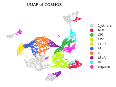
UMAP visualization of COSMOS integration
[6]:
# UMAP visualization
umap_2d = UMAP(n_components=2, init='random', random_state=random_seed, min_dist = 0.3,n_neighbors=30)
umap_pos = umap_2d.fit_transform(df_embedding)
adata_new.obs['cosmos_umap_pos_x'] = umap_pos[:,0]
adata_new.obs['cosmos_umap_pos_y'] = umap_pos[:,1]

# Ploting figures
matplotlib.rcParams['font.size'] = 8.0
fig, axes = plt.subplots(1, 1, figsize=(4,3))
sz = 10
domains="Cluster_cosmos"
num_celltype=len(adata_new.obs[domains].unique())
adata_new.uns[domains+"_colors"]=list(plot_color_1[:num_celltype])
titles = 'UMAP of COSMOS'
ax=sc.pl.scatter(adata_new,alpha=1,x="cosmos_umap_pos_x",y="cosmos_umap_pos_y",color=domains,title=titles ,color_map=plot_color_1,show=False,size=sz,ax = axes)
ax.axis('off')
plt.tight_layout()
Pseudo-spatiotemporal map (pSM) from COSMOS integration
[7]:
# Calculating pseudo-times
embedding_adata.uns['iroot'] = np.flatnonzero(adata_new.obs["Cluster_cosmos"] == 'CP2')[0]
sc.tl.diffmap(embedding_adata)
sc.tl.dpt(embedding_adata)
pSM_values_cosmos = embedding_adata.obs['dpt_pseudotime'].to_numpy()


# Ploting figures
matplotlib.rcParams['font.size'] = 8.0
fig, axes = plt.subplots(1, 1, figsize=(3,3))
sz = 10
x = np.array(adata_new.obs['x_pos'])
y = np.array(adata_new.obs['y_pos'])
ax_temp = axes
im = ax_temp.scatter(x, y, s=20, c=pSM_values_cosmos, marker='.', cmap='coolwarm',alpha = 1)
ax_temp.axis('off')
ax_temp.set_title('dpt_pseudotime of COSMOS')
plt.tight_layout()

Showing modality weights of two omics in COSMOS integration
[8]:
def plot_weight_value(alpha, label, modality1='RNA', modality2='ATAC',order = None):
    df = pd.DataFrame(columns=[modality1, modality2, 'label'])
    df[modality1], df[modality2] = alpha[:, 0], alpha[:, 1]
    df['label'] = label
    df = df.set_index('label').stack().reset_index()
    df.columns = ['label_COSMOS', 'Modality', 'Modality weights']
    matplotlib.rcParams['font.size'] = 8.0
    fig, axes = plt.subplots(1, 1, figsize=(5,3))
    ax = sns.violinplot(data=df, x='label_COSMOS', y='Modality weights', hue="Modality",
                split=True, inner="quart", linewidth=1, show=False, orient = 'v', order=order)
    plt.tight_layout(w_pad=0.05)
    ax.set_title(modality1 + ' vs ' + modality2)
    ax.set_xticklabels(order, rotation = 45)
ordered_cluster = np.unique(LayerName)
layer_type = ordered_cluster
index_all = [np.array([i for i in range(len(LayerName)) if LayerName[i] == ordered_cluster[0]])]
for k in range(1,len(layer_type)):
    temp_idx = np.array([i for i in range(len(LayerName)) if LayerName[i] == ordered_cluster[k]])
    index_all.append(temp_idx)

wghts_mean = np.mean(weights[index_all[0],:],0)
for k in range(1,len(ordered_cluster)):
    wghts_mean_temp = np.mean(weights[index_all[k],:],0)
    wghts_mean = np.vstack([wghts_mean, wghts_mean_temp])
df_wghts_mean = pd.DataFrame(wghts_mean,columns = ['w1','w2'],index = ordered_cluster)

df_sort_mean = df_wghts_mean.sort_values(by=['w1'])
plot_weight_value(weights, np.array(adata_new.obs['LayerName']), order = list(df_sort_mean.index))
